


Authors: Brian Schilder, Jack Humphrey, Towfique Raj
echolocatoR: Automated statistical and functional fine-mapping with extensive access to genome-wide datasets.
The echoverse
echolocatoR is part of the echoverse, a suite of R packages designed to facilitate different steps in genetic fine-mapping.
echolocatoR calls each of these other packages (i.e. “modules”) internally to create a unified pipeline. However, you can also use each module independently to create your own custom workflows.
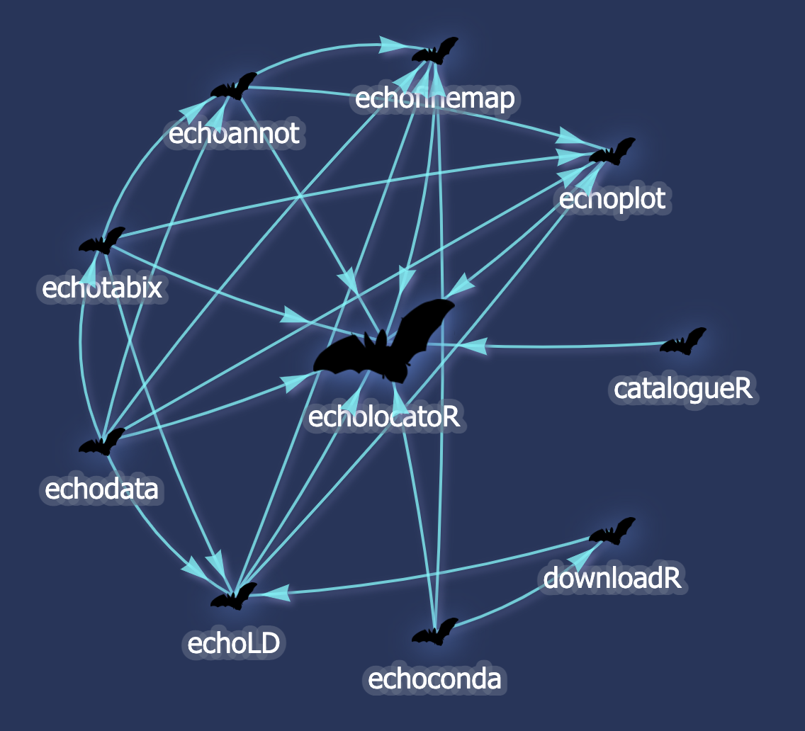
echoverse dependency graph
Made with
echodeps, yet another echoverse module. See here for the interactive version with package descriptions and links to each GitHub repo.
echoverse status
| Package | Level | Version | CI Status | Code Coverage | Runners |
|---|---|---|---|---|---|
| echolocatoR | 4 |  |
|
||
| catalogueR | 3 |  |
|
||
| echoAI | 3 |  |
|
||
| echoannot | 3 |  |
|
||
| echofinemap | 3 |  |
|
||
| echoplot | 3 |  |
|
||
| downloadR | 2 |  |
|
||
| echoconda | 2 |  |
|
||
| echoLD | 2 |  |
|
||
| echotabix | 2 |  |
|
||
| devoptera | 1 |  |
|
||
| echodata | 1 |  |
|
||
| echogithub | 1 |  |
|
||
| echodeps | - |  |
|
||
| echoverseTemplate | - |  |
|
Level indicates dependency depth: 4 = top-level pipeline, 3 = analysis modules, 2 = mid-level utilities, 1 = base packages, - = non-pipeline. CI status reflects all runners combined. Click the badge to see per-runner results.
Installation
Prerequisites
Before installing echolocatoR, make sure the following system libraries are available. These are needed to compile R packages that echolocatoR depends on.
macOS (via Homebrew):
Ubuntu / Debian:
Windows: Install Rtools matching your R version.
Install
if(!require("BiocManager")) install.packages("BiocManager")

BiocManager::install("RajLabMSSM/echolocatoR")
library(echolocatoR)
Diagnose issues
After installing, run the built-in diagnostic to check for any problems:
echolocatoR::check_echoverse_setup()Troubleshooting
-
Dependency ordering: Because
echolocatoRrelies on many subpackages that depend on one another, install errors can sometimes occur when R tries to update one package before its echoverse dependencies. The solution is to simply rerunBiocManager::install("RajLabMSSM/echolocatoR")until all subpackages are fully updated. -
susieR version:
echofinemaprequiressusieR>= 0.12.0, but CRAN sometimes has an older version. Fix:devtools::install_github("stephenslab/susieR") -
GitHub rate limiting: Installing many GitHub-hosted packages can trigger API rate limits. Set a GitHub Personal Access Token:
Sys.setenv(GITHUB_TOKEN = "your_token_here"). See GitHub docs for how to create one. -
Python / conda: Some fine-mapping methods (PolyFun) and LD reference panels (UKB) require Python and conda. Install Miniforge if you plan to use these features. The conda environment
echoR_miniwill be created automatically on first use.
[Optional] Docker/Singularity
echolocatoR now has its own dedicated Docker/Singularity container! This greatly reduces issues related to system dependency conflicts and provides a containerized interface for Rstudio through your web browser. See here for installation instructions.
Quick start
library(echolocatoR)

## Load bundled fine-mapping results for the BST1 locus
dat <- echodata::BST1

## View consensus fine-mapped SNPs (agreed upon by multiple methods)
subset(dat, Consensus_SNP == TRUE,
       select = c(SNP, CHR, POS, P, mean.PP, Support))

## Visualize the locus
echoplot::plot_locus(
    dat = dat,
    locus_dir = file.path(tempdir(), echodata::locus_dir),
    LD_matrix = echodata::BST1_LD_matrix
)
See vignette("echolocatoR") for the full pipeline, or vignette("explore_results") to learn how to interpret results.
Documentation
All echoverse vignettes
echoverse <- c('echolocatoR','echodata','echotabix',
               'echoannot','echoconda','echoLD',
               'echoplot','catalogueR','downloadR',
               'echofinemap','echodeps', # under construction
               'echogithub')
toc <- echogithub::github_pages_vignettes(owner = "RajLabMSSM",
                                          repo = echoverse,
                                          as_toc = TRUE,
verbose = FALSE)-
🦇 echolocatoR
-
🦇 echodata
-
🦇 echotabix
-
🦇 echoannot
-
🦇 echoconda
-
🦇 echoLD
-
🦇 echoplot
-
🦇 catalogueR
-
🦇 downloadR
-
🦇 echofinemap
-
🦇 echodeps
-
🦇 echogithub
-
NA
-
Introduction
Fine-mapping methods are a powerful means of identifying causal variants underlying a given phenotype, but are underutilized due to the technical challenges of implementation. echolocatoR is an R package that automates end-to-end genomics fine-mapping, annotation, and plotting in order to identify the most probable causal variants associated with a given phenotype.
It requires minimal input from users (a GWAS or QTL summary statistics file), and includes a suite of statistical and functional fine-mapping tools. It also includes extensive access to datasets (linkage disequilibrium panels, epigenomic and genome-wide annotations, QTL).
Citation
If you use echolocatoR, or any of the echoverse modules, please cite:
Brian M Schilder, Jack Humphrey, Towfique Raj (2021) echolocatoR: an automated end-to-end statistical and functional genomic fine-mapping pipeline, Bioinformatics; btab658, https://doi.org/10.1093/bioinformatics/btab658
The elimination of data gathering and preprocessing steps enables rapid fine-mapping of many loci in any phenotype, complete with locus-specific publication-ready figure generation. All results are merged into a single per-SNP summary file for additional downstream analysis and results sharing. Therefore echolocatoR drastically reduces the barriers to identifying causal variants by making the entire fine-mapping pipeline rapid, robust and scalable.

Literature
For applications of echolocatoR in the literature, please see:
- E Navarro, E Udine, K de Paiva Lopes, M Parks, G Riboldi, BM Schilder…T Raj (2020) Dysregulation of mitochondrial and proteo-lysosomal genes in Parkinson’s disease myeloid cells. Nature Genetics. https://doi.org/10.1101/2020.07.20.212407
- BM Schilder, T Raj (2021) Fine-Mapping of Parkinson’s Disease Susceptibility Loci Identifies Putative Causal Variants. Human Molecular Genetics, ddab294, https://doi.org/10.1093/hmg/ddab294
- K de Paiva Lopes, G JL Snijders, J Humphrey, A Allan, M Sneeboer, E Navarro, BM Schilder…T Raj (2022) Genetic analysis of the human microglial transcriptome across brain regions, aging and disease pathologies. Nature Genetics, https://doi.org/10.1038/s41588-021-00976-y
echolocatoR v1.0 vs. v2.0
There have been a series of major updates between echolocatoR v1.0 and v2.0. Here are some of the most notable ones (see Details):
-
echoverse subpackages:
echolocatoRhas been broken into separate subpackages, making it much easier to edit/debug each step of the fullfinemap_locipipeline, and improving robustness throughout. It also provides greater flexibility for users to construct their own custom pipelines from these modules. -
GITHUB_TOKEN: GitHub now requires users to create Personal Authentication Tokens (PAT) to avoid download limits. This is essential for installingecholocatoRas many resources from GitHub need to be downloaded. See here for further instructions. =echodata::construct_colmap(): Previously, users were required to input key column name mappings as separate arguments toecholocatoR::finemap_loci. This functionality has been deprecated and replaced with a single argument,colmap=. This allows users to save theconstruct_colmap()output as a single variable and reuse it later without having to write out each mapping argument again (and helps reduce an already crowded list of arguments). -
MungeSumstats:finemap_locinow accepts the output ofMungeSumstats::format_sumstats/import_sumstatsas-is (without requiringcolmap=, so long asmunged=TRUE). Standardizing your GWAS/QTL summary stats this way greatly reduces (or eliminates) the time taken to do manual formatting. -
echolocatoR::finemap_lociarguments: Several arguments have been deprecated or had their names changed to be harmonized across all the subpackages and use a unified naming convention. See?echolocatoR::finemap_locifor details. -
echoconda: The echoverse subpackageechocondanow handles all conda environment creation/use internally and automatically, without the need for users to create the conda environment themselves as a separate step. Also, the default conda envechoRhas been replaced byechoR_mini, which reduces the number of dependencies to just the bare minimum (thus greatly speeding up build time and reducing potential version conflicts). -
FINEMAP: More outputs from the toolFINEMAPare now recorded in theecholocatoRresults (see?echofinemap::FINEMAPor this Issue for details). Also, a common dependency conflict betweenFINEMAP>=1.4 and MacOS has been resolved (see this Issue for details. -
echodata: All example data and data transformation functions have been moved to the echoverse subpackageechodata. -
LD_reference=: In addition to the UKB, 1KGphase1/3 LD reference panels,finemap_loci()can now take custom LD panels by supplyingfinemap_loci(LD_reference=)with a list of paths to VCF files (.vcf / vcf.gz / vcf.bgz) or pre-computed LD matrices with RSIDs as the row/col names (.rda / .rds / .csv / .tsv. / .txt / .csv.gz / tsv.gz / txt.gz). - Expanded fine-mapping methods: “ABF”, “COJO_conditional”, “COJO_joint” “COJO_stepwise”,“FINEMAP”,“PAINTOR” (including multi-GWAS and multi-ancestry fine-mapping),“POLYFUN_FINEMAP” ,“POLYFUN_SUSIE”,“SUSIE”
-
FINEMAPfixed: There were a number of issues withFINEMAPdue to differing output formats across different versions, system dependency conflicts, and the fact that it can produce multiple Credible Sets. All of these have been fixed and the latest version ofFINEMAPcan be run on all OS platforms.
-
Debug mode: Within
finemap_loci()I use atryCatch()when iterating across loci so that if one locus fails, the rest can continue. However this prevents using traceback feature in R, making debugging hard. Thus I now enabled debugging mode via a new argument:use_tryCatch=FALSE.
Output descriptions
By default, echolocatoR::finemap_loci() returns a nested list containing grouped by locus names (e.g. $BST1, $MEX3C). The results of each locus contain the following elements:
-
finemap_dat: Fine-mapping results from all selected methods merged with the original summary statistics (i.e. Multi-finemap results). -
locus_plot: A nested list containing one or more zoomed views of locus plots.
-
LD_matrix: The post-processed LD matrix used for fine-mapping. -
LD_plot: An LD plot (if used). -
locus_dir: Locus directory results are saved in. -
arguments: A record of the arguments supplied tofinemap_loci.
In addition, the following object summarizes the results from the locus-specific elements:
- merged_dat: A merged data.table with all fine-mapping results from all loci.
Multi-finemap results files
The main output of echolocatoR are the multi-finemap files (for example, echodata::BST1). They are stored in the locus-specific Multi-finemap subfolders.
Column descriptions
-
Standardized GWAS/QTL summary statistics: e.g.
SNP,CHR,POS,Effect,StdErr. See?finemap_loci()for descriptions of each.
- leadSNP: The designated proxy SNP per locus, which is the SNP with the smallest p-value by default.
-
<tool>.CS: The 95% probability Credible Set (CS) to which a SNP belongs within a given fine-mapping tool’s results. If a SNP is not in any of the tool’s CS, it is assigned
NA(or0for the purposes of plotting).
-
<tool>.PP: The posterior probability that a SNP is causal for a given GWAS/QTL trait.
- Support: The total number of fine-mapping tools that include the SNP in its CS.
-
Consensus_SNP: By default, defined as a SNP that is included in the CS of more than
Nfine-mapping tool(s), i.e.Support>1(default:N=1).
- mean.PP: The mean SNP-wise PP across all fine-mapping tools used.
-
mean.CS: If mean PP is greater than the 95% probability threshold (
mean.PP>0.95) thenmean.CSis 1, else 0. This tends to be a very stringent threshold as it requires a high degree of agreement between fine-mapping tools.
Notes
- Separate multi-finemap files are generated for each LD reference panel used, which is included in the file name (e.g. UKB_LD.Multi-finemap.tsv.gz).
- Each fine-mapping tool defines its CS and PP slightly differently, so please refer to the associated original publications for the exact details of how these are calculated (links provided above).
Fine-mapping tools
Fine-mapping functions are now implemented via echofinemap:
-
echolocatoRwill automatically check whether you have the necessary columns to run each tool you selected inecholocatoR::finemap_loci(finemap_methods=...). It will remove any tools that for which there are missing necessary columns, and produces a message letting you know which columns are missing. - Note that some columns (e.g.
MAF,N,t-stat) will be automatically inferred if missing.
- For easy reference, we list the necessary columns here as well.
See?echodata::construct_colmap()for descriptions of these columns.
All methods require the columns:SNP,CHR,POS,Effect,StdErr
fm_methods <- echofinemap::required_cols(add_versions = FALSE,
                                         embed_links = TRUE,
                                         verbose = FALSE)
knitr::kable(x = fm_methods)| method | required | suggested | source | citation |
|---|---|---|---|---|
| ABF | SNP, CHR…. | source | cite | |
| COJO_conditional | SNP, CHR…. | Freq, P, N | source | cite |
| COJO_joint | SNP, CHR…. | Freq, P, N | source | cite |
| COJO_stepwise | SNP, CHR…. | Freq, P, N | source | cite |
| FINEMAP | SNP, CHR…. | A1, A2, …. | source | cite |
| PAINTOR | SNP, CHR…. | MAF | source | cite |
| POLYFUN_FINEMAP | SNP, CHR…. | MAF, N | source | cite |
| POLYFUN_SUSIE | SNP, CHR…. | MAF, N | source | cite |
| SUSIE | SNP, CHR…. | N | source | cite |
Datasets
Datasets are now stored/retrieved via the following echoverse subpackages:
- echodata: Pre-computed fine-mapping results. Also handles the semi-automated standardization of summary statistics.
- echoannot: Annotates GWAS/QTL summary statistics using epigenomics, pre-compiled annotation matrices, and machine learning model predictions of variant-specific functional impacts.
- catalogueR: Large compendium of fully standardized e/s/t-QTL summary statistics.
For more detailed information about each dataset, use ?:
### Examples ###

library(echoannot)
?NOTT_2019.interactome # epigenomic annotations
library(echodata)
?BST1 # fine-mapping results
MungeSumstats:
- You can search, import, and standardize any GWAS in the Open GWAS database via
MungeSumstats, specifically the functionsfind_sumstatsandimport_sumstats.
catalogueR: QTLs
eQTL Catalogue: catalogueR::eQTL_Catalogue.query()
- API access to full summary statistics from many standardized e/s/t-QTL datasets.
- Data access and colocalization tests facilitated through the
catalogueRR package.
echodata: fine-mapping results
echolocatoR Fine-mapping Portal: pre-computed fine-mapping results
- You can visit the echolocatoR Fine-mapping Portal to interactively visualize and download pre-computed fine-mapping results across a variety of phenotypes.
- This data can be searched and imported programmatically using
echodata::portal_query().
echoannot: Epigenomic & genome-wide annotations
Nott et al. (2019): echoannot::NOTT2019_*()
- Data from this publication contains results from cell type-specific (neurons, oligodendrocytes, astrocytes, microglia, & peripheral myeloid cells) epigenomic assays (H3K27ac, ATAC, H3K4me3) from ex vivo pediatric human brain tissue.
Corces et al.2020: echoannot::CORCES2020_*()
- Data from this publication contains results from single-cell and bulk chromatin accessibility assays ([sc]ATAC-seq) and chromatin interactions (
FitHiChIP) from postmortem adult human brain tissue.
XGR: echoannot::XGR_download_and_standardize()
- API access to a diverse library of cell type/line-specific epigenomic (e.g. ENCODE) and other genome-wide annotations.
Roadmap: echoannot::ROADMAP_query()
- API access to cell type-specific epigenomic data.
biomaRt: echoannot::annotate_snps()
- API access to various genome-wide SNP annotations (e.g. missense, nonsynonmous, intronic, enhancer).
HaploR: echoannot::annotate_snps()
- API access to known per-SNP QTL and epigenomic data hits.
Enrichment tools
Annotation enrichment functions are now implemented via echoannot:
Implemented
XGR: echoannot::XGR_enrichment()
- Binomial enrichment tests between customisable foreground and background SNPs.
motifbreakR: echoannot::MOTIFBREAKR()
- Identification of transcript factor binding motifs (TFBM) and prediction of SNP disruption to said motifs.
- Includes a comprehensive list of TFBM databases via MotifDB (9,900+ annotated position frequency matrices from 14 public sources, for multiple organisms).
regioneR: echoannot::test_enrichment()
- Iterative pairwise permutation testing of overlap between all combinations of two
GRangesListobjects.
Under construction
GARFIELD
- Genomic enrichment with LD-informed heuristics.
GoShifter
- LD-informed iterative enrichment analysis.
S-LDSC
- Genome-wide stratified LD score regression.
- Inlccles 187-annotation baseline model from Gazal et al. 2018.
- You can alternatively supply a custom annotations matrix.
LD reference panels
LD reference panels are now queried/processed by echoLD, specifically the function get_LD():
Plotting
Plotting functions are now implemented via:
- echoplot: Multi-track locus plots with GWAS, fine-mapping results, and functional annotations (plot_locus()). Can also plot multi-GWAS/QTL and multi-ancestry results (plot_locus_multi()).
- echoannot: Study-level summary plots showing aggregted info across many loci at once (super_summary_plot()).
- echoLD: Plot an LD matrix using one of several differnt plotting methods (plot_LD()).
Tabix queries
All queries of tabix-indexed files (for rapid data subset extraction) are implemented via echotabix.
-
echotabix::convert_and_query()detects whether the GWAS summary statistics file you provided is alreadytabix-indexed, and it not, automatically performs all steps necessary to convert it (sorting,bgzip-compression, indexing) across a wide variety of scenarios.
-
echotabix::query()contains many different methods for making tabix queries (e.g.Rtracklayer,echoconda,VariantAnnotation,seqminer), each of which fail in certain circumstances. To avoid this,query()automatically selects the method that will work for the particular file being queried and your machine’s particular versions of R/Bioconductor/OS, taking the guesswork and troubleshooting out oftabixqueries.
Downloads
Single- and multi-threaded downloads are now implemented via downloadR.
- Multi-threaded downloading is performed using
axel, and is particularly useful for speeding up downloads of large files. -
axelis installed via the official echoverse conda environment: “echoR_mini”. This environment is automatically created by the functionechoconda::yaml_to_env()when needed.
Brian M. Schilder, Bioinformatician II
Raj Lab
Department of Neuroscience, Icahn School of Medicine at Mount Sinai
Session info
utils::sessionInfo()## R version 4.5.1 (2025-06-13)
## Platform: aarch64-apple-darwin20
## Running under: macOS Tahoe 26.3.1
##
## Matrix products: default
## BLAS: /Library/Frameworks/R.framework/Versions/4.5-arm64/Resources/lib/libRblas.0.dylib
## LAPACK: /Library/Frameworks/R.framework/Versions/4.5-arm64/Resources/lib/libRlapack.dylib; LAPACK version 3.12.1
##
## locale:
## [1] en_US.UTF-8/en_US.UTF-8/en_US.UTF-8/C/en_US.UTF-8/en_US.UTF-8
##
## time zone: America/New_York
## tzcode source: internal
##
## attached base packages:
## [1] stats graphics grDevices utils datasets methods base
##
## loaded via a namespace (and not attached):
## [1] splines_4.5.1 aws.s3_0.3.22
## [3] BiocIO_1.20.0 bitops_1.0-9
## [5] filelock_1.0.3 cellranger_1.1.0
## [7] tibble_3.3.1 R.oo_1.27.1
## [9] basilisk.utils_1.22.0 graph_1.88.1
## [11] rpart_4.1.24 XML_3.99-0.22
## [13] lifecycle_1.0.5 httr2_1.2.2
## [15] mixsqp_0.3-54 rprojroot_2.1.1
## [17] OrganismDbi_1.52.0 ensembldb_2.34.0
## [19] lattice_0.22-9 MASS_7.3-65
## [21] backports_1.5.0 magrittr_2.0.4
## [23] Hmisc_5.2-5 openxlsx_4.2.8.1
## [25] rmarkdown_2.30 yaml_2.3.12
## [27] dlstats_0.1.7 otel_0.2.0
## [29] zip_2.3.3 ggbio_1.58.0
## [31] reticulate_1.45.0 gld_2.6.8
## [33] DBI_1.3.0 RColorBrewer_1.1-3
## [35] abind_1.4-8 expm_1.0-0
## [37] rvcheck_0.2.1 GenomicRanges_1.62.1
## [39] purrr_1.2.1 R.utils_2.13.0
## [41] AnnotationFilter_1.34.0 biovizBase_1.58.0
## [43] BiocGenerics_0.56.0 RCurl_1.98-1.17
## [45] nnet_7.3-20 yulab.utils_0.2.4
## [47] VariantAnnotation_1.56.0 rappdirs_0.3.4
## [49] rworkflows_1.0.8 IRanges_2.44.0
## [51] S4Vectors_0.48.0 echoLD_0.99.12
## [53] echofinemap_1.0.0 irlba_2.3.7
## [55] gitcreds_0.1.2 echodata_1.0.0
## [57] piggyback_0.1.5 codetools_0.2-20
## [59] DelayedArray_0.36.0 DT_0.34.0
## [61] xml2_1.5.2 tidyselect_1.2.1
## [63] UCSC.utils_1.6.1 farver_2.1.2
## [65] viridis_0.6.5 matrixStats_1.5.0
## [67] stats4_4.5.1 base64enc_0.1-6
## [69] Seqinfo_1.0.0 echotabix_1.0.0
## [71] GenomicAlignments_1.46.0 jsonlite_2.0.0
## [73] e1071_1.7-17 Formula_1.2-5
## [75] survival_3.8-6 tools_4.5.1
## [77] DescTools_0.99.60 Rcpp_1.1.1
## [79] glue_1.8.0 gridExtra_2.3
## [81] SparseArray_1.10.9 xfun_0.56
## [83] here_1.0.2 MatrixGenerics_1.22.0
## [85] GenomeInfoDb_1.46.2 dplyr_1.2.0
## [87] withr_3.0.2 BiocManager_1.30.27
## [89] fastmap_1.2.0 basilisk_1.22.0
## [91] boot_1.3-32 digest_0.6.39
## [93] R6_2.6.1 colorspace_2.1-2
## [95] dichromat_2.0-0.1 RSQLite_2.4.6
## [97] cigarillo_1.0.0 R.methodsS3_1.8.2
## [99] tidyr_1.3.2 generics_0.1.4
## [101] renv_1.1.8 data.table_1.18.2.1
## [103] rtracklayer_1.70.1 class_7.3-23
## [105] httr_1.4.8 htmlwidgets_1.6.4
## [107] S4Arrays_1.10.1 pkgconfig_2.0.3
## [109] gtable_0.3.6 Exact_3.3
## [111] blob_1.3.0 S7_0.2.1
## [113] XVector_0.50.0 echoconda_1.0.0
## [115] htmltools_0.5.9 susieR_0.14.2
## [117] RBGL_1.86.0 ProtGenerics_1.42.0
## [119] scales_1.4.0 Biobase_2.70.0
## [121] lmom_3.2 png_0.1-8
## [123] knitr_1.51 rstudioapi_0.18.0
## [125] reshape2_1.4.5 tzdb_0.5.0
## [127] rjson_0.2.23 checkmate_2.3.4
## [129] badger_0.2.5 curl_7.0.0
## [131] proxy_0.4-29 cachem_1.1.0
## [133] stringr_1.6.0 rootSolve_1.8.2.4
## [135] parallel_4.5.1 foreign_0.8-91
## [137] AnnotationDbi_1.72.0 restfulr_0.0.16
## [139] desc_1.4.3 pillar_1.11.1
## [141] grid_4.5.1 reshape_0.8.10
## [143] vctrs_0.7.1 cluster_2.1.8.2
## [145] htmlTable_2.4.3 evaluate_1.0.5
## [147] readr_2.2.0 GenomicFeatures_1.62.0
## [149] mvtnorm_1.3-3 cli_3.6.5
## [151] compiler_4.5.1 echogithub_0.99.5
## [153] Rsamtools_2.26.0 rlang_1.1.7
## [155] crayon_1.5.3 aws.signature_0.6.0
## [157] forcats_1.0.1 plyr_1.8.9
## [159] fs_1.6.7 stringi_1.8.7
## [161] coloc_5.2.3 echoannot_1.0.1
## [163] viridisLite_0.4.3 BiocParallel_1.44.0
## [165] Biostrings_2.78.0 lazyeval_0.2.2
## [167] gh_1.5.0 Matrix_1.7-4
## [169] downloadR_1.0.0 dir.expiry_1.18.0
## [171] BSgenome_1.78.0 patchwork_1.3.2
## [173] hms_1.1.4 bit64_4.6.0-1
## [175] ggplot2_4.0.2 KEGGREST_1.50.0
## [177] haven_2.5.5 SummarizedExperiment_1.40.0
## [179] memoise_2.0.1 snpStats_1.60.0
## [181] bit_4.6.0 readxl_1.4.5