Generate a locus plot — plot

Generate a locus-specific plot with multiple selectable tracks. Users can also generate multiple zoomed in views of the plot at multiple resolutions.

Usage

plot_locus(
  dat,
  locus_dir,
  LD_matrix = NULL,
  LD_reference = NULL,
  facet_formula = "Method~.",
  dataset_type = "GWAS",
  color_r2 = TRUE,
  finemap_methods = c("ABF", "FINEMAP", "SUSIE", "POLYFUN_SUSIE"),
  track_order = NULL,
  track_heights = NULL,
  plot_full_window = TRUE,
  dot_summary = FALSE,
  qtl_suffixes = NULL,
  mean.PP = TRUE,
  credset_thresh = 0.95,
  consensus_thresh = 2,
  sig_cutoff = 5e-08,
  gene_track = TRUE,
  tx_biotypes = NULL,
  point_size = 1,
  point_alpha = 0.6,
  density_adjust = 0.2,
  snp_group_lines = c("Lead", "UCS", "Consensus"),
  labels_subset = c("Lead", "CS", "Consensus"),
  xtext = FALSE,
  show_legend_genes = TRUE,
  xgr_libnames = NULL,
  xgr_n_top = 5,
  roadmap = FALSE,
  roadmap_query = NULL,
  roadmap_n_top = 7,
  zoom_exceptions_str = "*full window$|zoom_polygon",
  nott_epigenome = FALSE,
  nott_regulatory_rects = TRUE,
  nott_show_placseq = TRUE,
  nott_binwidth = 200,
  nott_bigwig_dir = NULL,
  save_plot = FALSE,
  show_plot = TRUE,
  genomic_units = "Mb",
  strip.text.y.angle = 0,
  max_transcripts = 1,
  zoom = c("1x"),
  dpi = 300,
  height = 12,
  width = 10,
  plot_format = "png",
  save_RDS = FALSE,
  return_list = FALSE,
  conda_env = "echoR_mini",
  nThread = 1,
  verbose = TRUE
)

Arguments

dat

Data to query transcripts with.

locus_dir

Storage directory to use.

LD_matrix

LD matrix.

LD_reference

LD reference to use:

1KGphase1: 1000 Genomes Project Phase 1 (genome build: hg19).
1KGphase3: 1000 Genomes Project Phase 3 (genome build: hg19).
UKB: Pre-computed LD from a British European-decent subset of UK Biobank. Genome build : hg19
<vcf_path>: User-supplied path to a custom VCF file to compute LD matrix from.
Accepted formats: .vcf / .vcf.gz / .vcf.bgz
Genome build : defined by user with target_genome.
<matrix_path>: User-supplied path to a pre-computed LD matrix. Accepted formats: .rds / .rda / .csv / .tsv / .txt
Genome build : defined by user with target_genome.

facet_formula

Formula to facet plots by. See facet_grid for details.

dataset_type

Dataset type (e.g. "GWAS" or "eQTL").

color_r2

Whether to color data points (SNPs) by how strongly they correlate with the lead SNP (i.g. LD measured in terms of r2).

finemap_methods

Fine-mapping methods to plot tracks for, where the y-axis show the Posterior Probabilities (PP) of each SNP being causal.

track_order

The order in which tracks should appear (from top to bottom).

track_heights

The height of each track (from top to bottom).

plot_full_window

Include a track with a Manhattan plot of the full GWAS/eQTL locus (not just the zoomed-in portion).

dot_summary

Include a dot-summary plot that highlights the Lead, Credible Set, and Consensus SNPs.

qtl_suffixes

If columns with QTL data is included in dat, you can indicate which columns those are with one or more string suffixes (e.g. qtl_suffixes=c(".eQTL1",".eQTL2") to use the columns "P.QTL1", "Effect.QTL1", "P.QTL2", "Effect.QTL2").

mean.PP

Include a track showing mean Posterior Probabilities (PP) averaged across all fine-mapping methods.

credset_thresh

The minimum fine-mapped posterior probability for a SNP to be considered part of a Credible Set. For example, credset_thresh=.95 means that all Credible Set SNPs will be 95% Credible Set SNPs.

consensus_thresh

The minimum number of fine-mapping tools in which a SNP is in the Credible Set in order to be included in the "Consensus_SNP" column.

sig_cutoff

Filters out SNPs to plot based on an (uncorrected) p-value significance cutoff.

gene_track

Include a track showing gene bodies.

tx_biotypes

Transcript biotypes to include in the gene model track. By default (NULL), all transcript biotypes will be included. See get_tx_biotypes for a full list of all available biotypes

point_size

Size of each data point.

point_alpha

Opacity of each data point.

density_adjust

Passed to adjust argument in geom_density.

snp_group_lines

Include vertical lines to help highlight SNPs belonging to one or more of the following groups: Lead, Credible Set, Consensus.

labels_subset

Include colored shapes and RSID labels to help highlight SNPs belonging to one or more of the following groups: Lead, Credible Set, Consensus.

xtext

Include x-axis title and text for each track (not just the lower-most one).

show_legend_genes

Show the legend for the gene_track.

xgr_libnames

Passed to XGR_plot. Which XGR annotations to check overlap with. For full list of libraries see here (XGR on CRAN). Passed to the RData.customised argument in XGR::xRDataLoader. Examples:

"ENCODE_TFBS_ClusteredV3_CellTypes"
"ENCODE_DNaseI_ClusteredV3_CellTypes"
"Broad_Histone"

xgr_n_top

Passed to XGR_plot. Number of top annotations to be plotted (passed to XGR_filter_sources and then XGR_filter_assays).

roadmap

Find and plot annotations from Roadmap.

roadmap_query

Only plot annotations from Roadmap whose metadata contains a string or any items from a list of strings (e.g. "brain" or c("brain","liver","monocytes")).

roadmap_n_top

Passed to ROADMAP_plot. Number of top annotations to be plotted (passed to ROADMAP_query).

zoom_exceptions_str

Names of tracks to exclude when zooming.

nott_epigenome

Include tracks showing brain cell-type-specific epigenomic data from Nott et al. (2019) (doi:10.1126/science.aay0793 ).

nott_regulatory_rects

Include track generated by NOTT2019_epigenomic_histograms.

nott_show_placseq

Include track generated by NOTT2019_plac_seq_plot.

nott_binwidth

When including Nott et al. (2019) epigenomic data in the track plots, adjust the bin width of the histograms.

nott_bigwig_dir

Instead of pulling Nott et al. (2019) epigenomic data from the UCSC Genome Browser, use a set of local bigwig files.

save_plot

Save plot as RDS file.

show_plot

Print plot to screen.

genomic_units

Which genomic units to return window limits in.

strip.text.y.angle

Angle of the y-axis facet labels.

max_transcripts

Maximum number of transcripts per gene.

zoom

Zoom into the center of the locus when plotting (without editing the fine-mapping results file). You can provide either:

The size of your plot window in terms of basepairs (e.g. zoom=50000 for a 50kb window).
How much you want to zoom in (e.g. zoom="1x" for the full locus, zoom="2x" for 2x zoom into the center of the locus, etc.).

You can pass a list of window sizes (e.g. c(50000,100000,500000)) to automatically generate multiple views of each locus. This can even be a mix of different style inputs: e.g. c("1x","4.5x",25000).

dpi

dpi to use for raster graphics

height

height (defaults to the height of current plotting window)

width

width (defaults to the width of current plotting window)

plot_format

Format to save plot as when saving with ggsave.

save_RDS

Save the tracks as an RDS file (Warning: These plots take up a lot disk space).

return_list

Return a named list with each track as a separate plot (default: FALSE). If TRUE, will return a merged plot using wrap_plots.

conda_env

Conda environment to use.

nThread

Number of threads to parallelise across (when applicable).

verbose

Print messages.

Examples

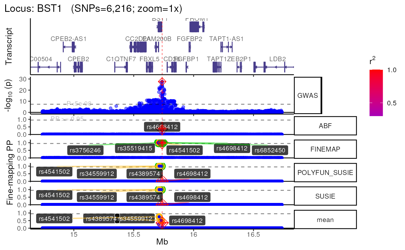
dat1 <- echodata::BST1
LD_matrix <- echodata::BST1_LD_matrix
locus_dir <- file.path(tempdir(),echodata::locus_dir)
plt <- echoplot::plot_locus(dat = dat1,
                            locus_dir = locus_dir,
                            LD_matrix = LD_matrix,
                            show_plot = TRUE)
#> +-------- Locus Plot:  BST1 --------+
#> + support_thresh = 2
#> + Calculating mean Posterior Probability (mean.PP)...
#> + 4 fine-mapping methods used.
#> + 7 Credible Set SNPs identified.
#> + 3 Consensus SNPs identified.
#> + Filling NAs in CS cols with 0.
#> + Filling NAs in PP cols with 0.
#> LD_matrix detected. Coloring SNPs by LD with lead SNP.
#> Filling r/r2 NAs with 0
#> ++ echoplot:: GWAS full window track
#> ++ echoplot:: GWAS track
#> ++ echoplot:: Merged fine-mapping track
#> Melting PP and CS from 5 fine-mapping methods.
#> + echoplot:: Constructing SNP labels.
#> Data is already melted. Skipping.
#> Loading required namespace: ggrepel
#> Adding SNP group labels to locus plot.
#> ++ echoplot:: Adding Gene model track.
#> Converting dat to GRanges object.
#> max_transcripts= 1 . 
#> 16  transcripts from  16  genes returned.
#> Fetching data...
#> OK
#> Parsing exons...
#> OK
#> Defining introns...
#> OK
#> Defining UTRs...
#> OK
#> Defining CDS...
#> OK
#> aggregating...
#> Done
#> Constructing graphics...
#> + Adding vertical lines to highlight SNP groups.
#> +>+>+>+>+ zoom =  1x  +<+<+<+<+
#> + echoplot:: Get window suffix...
#> + echoplot:: Removing GWAS full window track @ zoom=1x
#> + Removing subplot margins...
#> + Reordering tracks...
#> + Ensuring last track shows genomic units.
#> + Aligning xlimits for each subplot...
#> + Checking track heights...