catalogueR: colocalize
Brian M. Schilder
Most recent update:
2021-02-20
Source: vignettes/colocalize.Rmd
colocalize.RmdTutorial: Colocalize
library(catalogueR)
library(dplyr)
#>
#> Attaching package: 'dplyr'
#> The following objects are masked from 'package:stats':
#>
#>     filter, lag
#> The following objects are masked from 'package:base':
#>
#>     intersect, setdiff, setequal, union
Introduction
Here, we aim to more robustly test whether the genetic signals underlying two dataset (e.g. GWAS vs. eQTL in the same locus)are indeed the same, using a methodology called colocalization.
Specifically, we will use
coloc, which infers the probability that each SNP is causal in a given locus in each of the datasets. It then tests the hypothesis that those signals show substantially similar association distributions.
List datasets
We have previously queried eQTL Catalogue using several Parkinson’s disease GWAS loci (with
eQTL_Catalogue.query()).Let’s first gather those files and save them to disk as csv files.
query_res <- list("BST1"=catalogueR::BST1__Alasoo_2018.macrophage_IFNg,
                  "LRRK2"=catalogueR::LRRK2__Alasoo_2018.macrophage_IFNg,
                   "MEX3C"=catalogueR::MEX3C__Alasoo_2018.macrophage_IFNg
)

# select where you want to store them
storage_dir <- "catalogueR_queries/Nalls23andMe_2019"

gwas.qtl_paths <- lapply(names(query_res), function(x){
  storage_path <- file.path(storage_dir,
                            "Alasoo_2018.macrophage_IFNg",
                            paste0(x,"__Alasoo_2018.macrophage_IFNg.tsv.gz"))
  dir.create(dirname(storage_path), showWarnings = F, recursive = T)
  data.table::fwrite(query_res[[x]], storage_path)
  return(storage_path)
}) %>%unlist() %>% `names<-`(names(query_res))
Run coloc
- Since its original release,
colochas been updated so that it can now model multiple causal variants within a given dataset (see the paper), whereas previously it could assume one causal variants. Thus, it may be able to better estimate the colocalization probability between two datasets.
coloc_QTLs <- run_coloc(gwas.qtl_paths,
                        save_path="./coloc_results.tsv.gz",
                        nThread=4,
                        top_snp_only=T,
                        split_by_group=F,
                        method = "abf")
#> + QTL Group = Alasoo_2018.macrophage_IFNg
Plot results
First, let’s plot only the results with >80% colocalization probability. This is a colocalization threshold commonly used in the field.
coloc_plot <- plot_coloc_summary(coloc_QTLs = coloc_QTLs,
                                 PP_thresh = .8)
#> Error in plot_coloc_summary(coloc_QTLs = coloc_QTLs, PP_thresh = 0.8):
#>
#> ** No coloc tests reached the PPH4 threshold (0.8).Try lowering `PP_thresh`. **
Uh oh! Looks like there were no colocalizations at 80% probability. Let’s explore the data a bit and lower the threshold.
Indeed, two loci show mild colocalization at 50% probability. As a general rule, the more tests you do to higher your probability threshold should be, since Bayesian methods don’t calculate P-values (and this cannot used multiple-testing correction methods like FDR).
For example, if you ran many thousands of coloc test across many GWAS-eQTL pairs, it’s advisable to raise your PP threshold to .90 or even .99. This also has the benefit of narrowing down your (sometimes many!) results so that you may focus on only the strongest colocalizations.
coloc_plot <- plot_coloc_summary(coloc_QTLs = coloc_QTLs,
                                 PP_thresh = .5)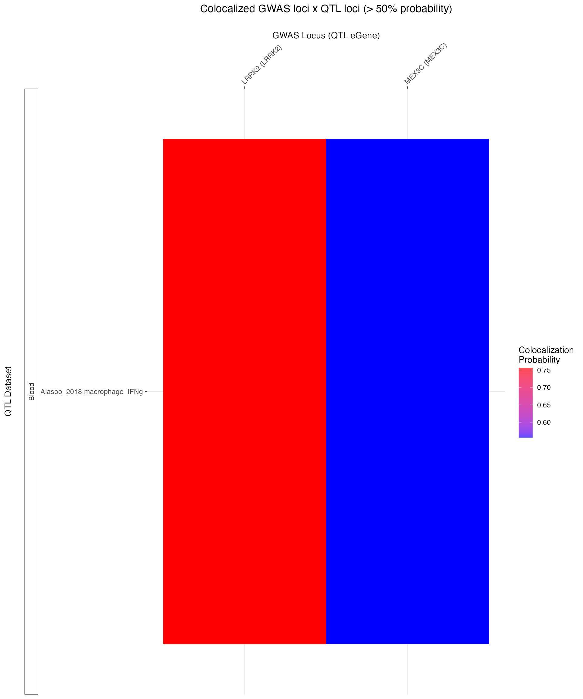
Session info
utils::sessionInfo()
#> R version 4.0.3 (2020-10-10)
#> Platform: x86_64-apple-darwin17.0 (64-bit)
#> Running under: macOS Big Sur 10.16
#>
#> Matrix products: default
#> BLAS:   /Library/Frameworks/R.framework/Versions/4.0/Resources/lib/libRblas.dylib
#> LAPACK: /Library/Frameworks/R.framework/Versions/4.0/Resources/lib/libRlapack.dylib
#>
#> locale:
#> [1] en_GB.UTF-8/en_GB.UTF-8/en_GB.UTF-8/C/en_GB.UTF-8/en_GB.UTF-8
#>
#> attached base packages:
#> [1] stats     graphics  grDevices utils     datasets  methods   base
#>
#> other attached packages:
#> [1] dplyr_1.0.4      catalogueR_0.1.0
#>
#> loaded via a namespace (and not attached):
#>  [1] highr_0.8         compiler_4.0.3    pillar_1.4.7      tools_4.0.3
#>  [5] digest_0.6.27     evaluate_0.14     memoise_2.0.0     lifecycle_1.0.0
#>  [9] tibble_3.0.6      gtable_0.3.0      pkgconfig_2.0.3   rlang_0.4.10
#> [13] DBI_1.1.1         parallel_4.0.3    yaml_2.2.1        pkgdown_1.6.1
#> [17] xfun_0.21         fastmap_1.1.0     stringr_1.4.0     knitr_1.31
#> [21] generics_0.1.0    desc_1.2.0        fs_1.5.0          vctrs_0.3.6
#> [25] systemfonts_1.0.1 rprojroot_2.0.2   grid_4.0.3        tidyselect_1.1.0
#> [29] glue_1.4.2        data.table_1.13.6 R6_2.5.0          textshaping_0.3.0
#> [33] rmarkdown_2.6     farver_2.0.3      tidyr_1.1.2       purrr_0.3.4
#> [37] ggplot2_3.3.3     magrittr_2.0.1    scales_1.1.1      htmltools_0.5.1.1
#> [41] ellipsis_0.3.1    assertthat_0.2.1  colorspace_2.0-0  labeling_0.4.2
#> [45] ragg_1.1.0        stringi_1.5.3     munsell_0.5.0     cachem_1.0.3
#> [49] crayon_1.4.1