Plotting fine-mapping results
Author: Brian M. Schilder
Author: Brian M. Schilder
Updated: Mar-16-2026
Source: Updated: Mar-16-2026
vignettes/plotting.Rmd
plotting.Rmd## ## ── 🦇 🦇 🦇 e c h o l o c a t o R 🦇 🦇 🦇 ─────────────────────────────────## ## ── v2.0.5 ──────────────────────────────────────────────────────────────────────## ## ────────────────────────────────────────────────────────────────────────────────## ⠊⠉⠡⣀⣀⠊⠉⠡⣀⣀⠊⠉⠢⣀⡠⠊⠉⠢⣀⡠⠊⠉⠢⣀⡠⠊⠉⠢⣀⡠⠊⠉⠢⣀⡠⠊⠉⠢⣀⡠
## ⠌⢁⡐⠉⣀⠊⢂⡐⠑⣀⠊⢂⡐⠑⣀⠊⢂⡐⠑⣀⠊⢂⡐⠑⣀⠊⢂⡐⠑⣀⠉⢂⡈⠑⣀⠉⢄⡈⠡⣀
## ⠌⡈⡐⢂⢁⠒⡈⡐⢂⢁⠒⡈⡐⢂⢁⠑⡈⡈⢄⢁⠡⠌⡈⠤⢁⠡⠌⡈⠤⢁⠡⠌⡈⡠⢁⢁⠊⡈⡐⢂
## ⠌⡈⡐⢂⢁⠒⡈⡐⢂⢁⠒⡈⡐⢂⢁⠑⡈⡈⢄⢁⠡⠌⡈⠤⢁⠡⠌⡈⠤⢁⠡⠌⡈⡠⢁⢁⠊⡈⡐⢂
## ⠌⢁⡐⠉⣀⠊⢂⡐⠑⣀⠊⢂⡐⠑⣀⠊⢂⡐⠑⣀⠊⢂⡐⠑⣀⠊⢂⡐⠑⣀⠉⢂⡈⠑⣀⠉⢄⡈⠡⣀
## ⠊⠉⠡⣀⣀⠊⠉⠡⣀⣀⠊⠉⠢⣀⡠⠊⠉⠢⣀⡠⠊⠉⠢⣀⡠⠊⠉⠢⣀⡠⠊⠉⠢⣀⡠⠊⠉⠢⣀⡠
## ⓞ If you use echolocatoR or any of the echoverse subpackages, please cite:
## ▶ Brian M Schilder, Jack Humphrey, Towfique
## Raj (2021) echolocatoR: an automated
## end-to-end statistical and functional
## genomic fine-mapping pipeline,
## Bioinformatics; btab658,
## https://doi.org/10.1093/bioinformatics/btab658
## ⓞ Please report any bugs/feature requests on GitHub:
## ▶
## https://github.com/RajLabMSSM/echolocatoR/issues
## ⓞ Contributions are welcome!:
## ▶
## https://github.com/RajLabMSSM/echolocatoR/pulls
can_plot <- tryCatch({
    requireNamespace("echoplot", quietly = TRUE) &&
    requireNamespace("ggplot2", quietly = TRUE) &&
    requireNamespace("patchwork", quietly = TRUE)
}, error = function(e) FALSE)
Overview
echoplot provides multi-track locus plots that combine
GWAS association signals, fine-mapping posterior probabilities, LD
structure, and gene models in a single figure. This vignette
demonstrates common plotting workflows using bundled example data —
no internet connection is required.
For the full fine-mapping pipeline, see
vignette("echolocatoR"). For interpreting results, see
vignette("explore_results").
Load example data
dat <- echodata::BST1
LD_matrix <- echodata::BST1_LD_matrix
locus_dir <- file.path(tempdir(), echodata::locus_dir)
Basic locus plot
The main function echoplot::plot_locus() creates a
multi-panel figure with GWAS p-values, fine-mapping posterior
probabilities, and gene tracks. SNPs are colored by LD r² with the lead
SNP.
plt <- tryCatch(
    echoplot::plot_locus(
        dat = dat,
        locus_dir = locus_dir,
        LD_matrix = LD_matrix,
        show_plot = FALSE,
        save_plot = FALSE,
        verbose = FALSE
    ),
    error = function(e) { message("plot_locus error: ", e$message); NULL }
)
## + support_thresh = 2## + Calculating mean Posterior Probability (mean.PP)...## + 4 fine-mapping methods used.## + 7 Credible Set SNPs identified.## + 3 Consensus SNPs identified.## + Filling NAs in CS cols with 0.## + Filling NAs in PP cols with 0.## Loading required namespace: ggrepel## Loading required namespace: EnsDb.Hsapiens.v75## Fetching data...OK
## Parsing exons...OK
## Defining introns...OK
## Defining UTRs...OK
## Defining CDS...OK
## aggregating...
## Done
## Constructing graphics...
## + echoplot:: Get window suffix...
if (!is.null(plt)) plt[["1x"]]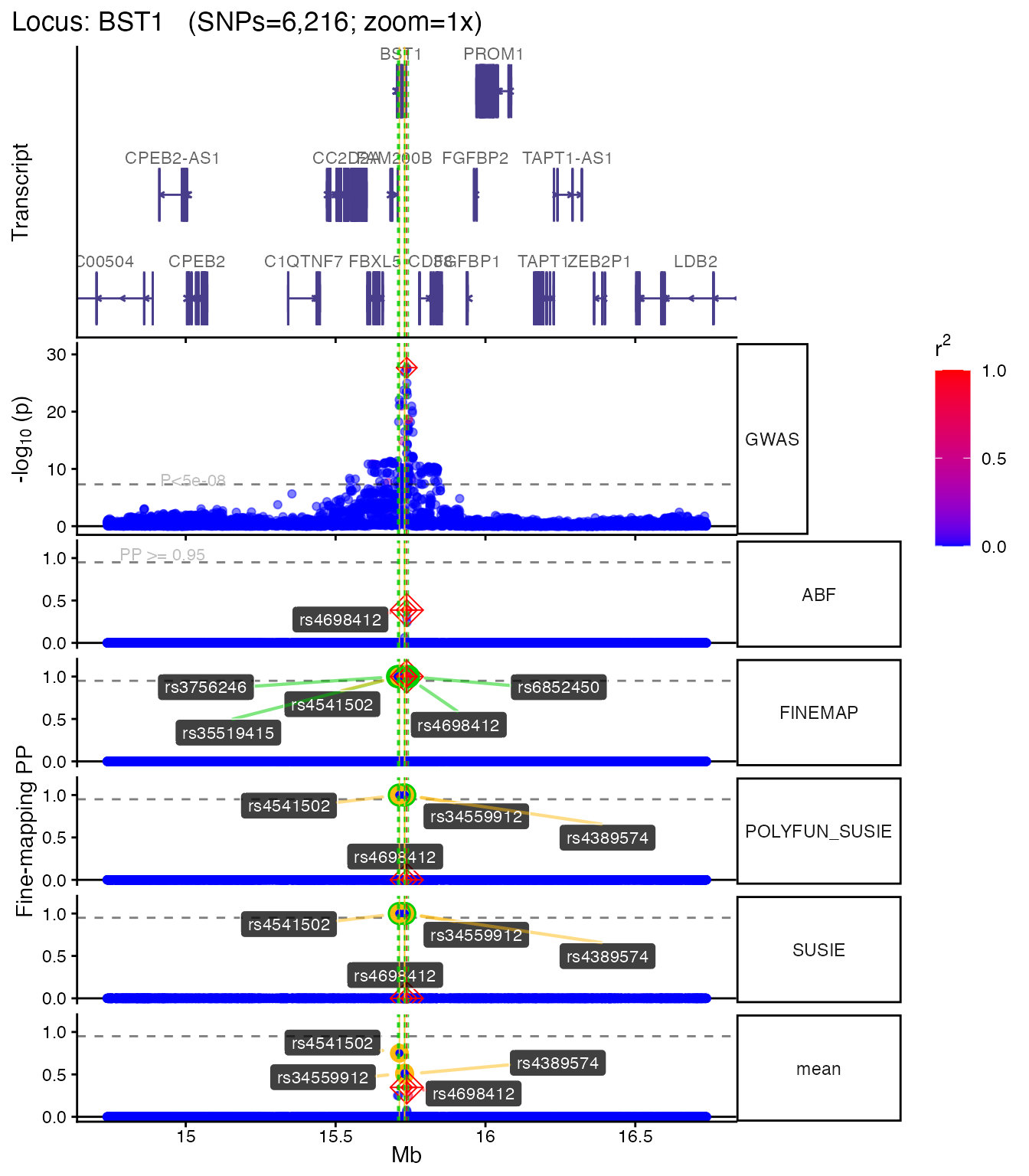
Customizing the plot
Multiple zoom levels
You can generate plots at different zoom levels to focus on the fine-mapped region:
plt_zoom <- tryCatch(
    echoplot::plot_locus(
        dat = dat,
        locus_dir = locus_dir,
        LD_matrix = LD_matrix,
        zoom = c("1x", "4x"),
        show_plot = FALSE,
        save_plot = FALSE,
        verbose = FALSE
    ),
    error = function(e) { message("plot_locus error: ", e$message); NULL }
)
## + support_thresh = 2## + Calculating mean Posterior Probability (mean.PP)...## + 4 fine-mapping methods used.## + 7 Credible Set SNPs identified.## + 3 Consensus SNPs identified.## + Filling NAs in CS cols with 0.## + Filling NAs in PP cols with 0.## Fetching data...OK
## Parsing exons...OK
## Defining introns...OK
## Defining UTRs...OK
## Defining CDS...OK
## aggregating...
## Done
## Constructing graphics...
## + echoplot:: Get window suffix...
## + echoplot:: Get window suffix...
## + Constructing zoom polygon...
## + Highlighting zoom origin...
if (!is.null(plt_zoom)) plt_zoom[["4x"]]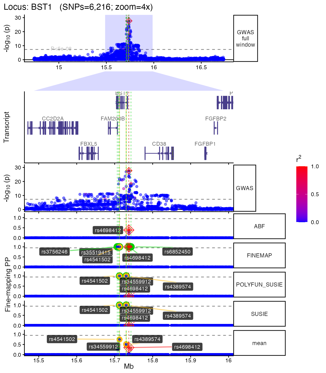
Without LD coloring
If you don’t have an LD matrix, the plot still works — SNPs are shown without r² coloring:
plt_nold <- tryCatch(
    echoplot::plot_locus(
        dat = dat,
        locus_dir = locus_dir,
        LD_matrix = NULL,
        show_plot = FALSE,
        save_plot = FALSE,
        verbose = FALSE
    ),
    error = function(e) { message("plot_locus error: ", e$message); NULL }
)
## + support_thresh = 2## + Calculating mean Posterior Probability (mean.PP)...## + 4 fine-mapping methods used.## + 7 Credible Set SNPs identified.## + 3 Consensus SNPs identified.## + Filling NAs in CS cols with 0.## + Filling NAs in PP cols with 0.## Fetching data...OK
## Parsing exons...OK
## Defining introns...OK
## Defining UTRs...OK
## Defining CDS...OK
## aggregating...
## Done
## Constructing graphics...
## + echoplot:: Get window suffix...
if (!is.null(plt_nold)) plt_nold[["1x"]]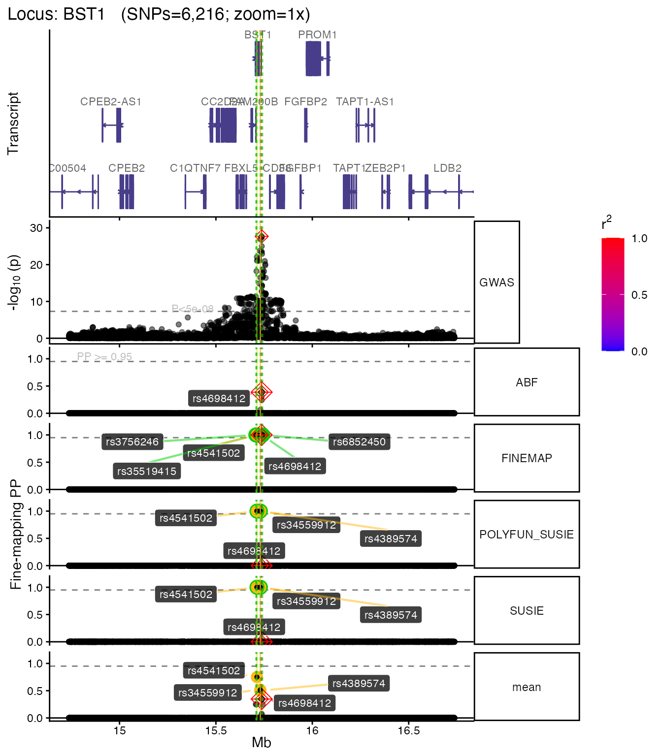
Saving plots
To save a plot to disk:
plt <- echoplot::plot_locus(
    dat = dat,
    locus_dir = locus_dir,
    LD_matrix = LD_matrix,
    save_plot = TRUE,
    plot_format = "png",
    dpi = 300,
    height = 12,
    width = 10,
    show_plot = FALSE
)
Next steps
- Fine-map your own loci:
vignette("echolocatoR") - Explore results in detail:
vignette("explore_results") - Summarise across loci:
vignette("summarise") - Learn about sub-packages:
vignette("echoverse_modules")
Session info
utils::sessionInfo()## R version 4.5.1 (2025-06-13)
## Platform: aarch64-apple-darwin20
## Running under: macOS Tahoe 26.3.1
##
## Matrix products: default
## BLAS: /Library/Frameworks/R.framework/Versions/4.5-arm64/Resources/lib/libRblas.0.dylib
## LAPACK: /Library/Frameworks/R.framework/Versions/4.5-arm64/Resources/lib/libRlapack.dylib; LAPACK version 3.12.1
##
## locale:
## [1] en_US.UTF-8/en_US.UTF-8/en_US.UTF-8/C/en_US.UTF-8/en_US.UTF-8
##
## time zone: America/New_York
## tzcode source: internal
##
## attached base packages:
## [1] stats graphics grDevices utils datasets methods base
##
## other attached packages:
## [1] echolocatoR_2.0.5 BiocStyle_2.38.0
##
## loaded via a namespace (and not attached):
## [1] splines_4.5.1 aws.s3_0.3.22
## [3] BiocIO_1.20.0 bitops_1.0-9
## [5] filelock_1.0.3 tibble_3.3.1
## [7] R.oo_1.27.1 cellranger_1.1.0
## [9] basilisk.utils_1.22.0 graph_1.88.1
## [11] rpart_4.1.24 XML_3.99-0.22
## [13] lifecycle_1.0.5 mixsqp_0.3-54
## [15] pals_1.10 OrganismDbi_1.52.0
## [17] ensembldb_2.34.0 lattice_0.22-9
## [19] MASS_7.3-65 backports_1.5.0
## [21] magrittr_2.0.4 Hmisc_5.2-5
## [23] openxlsx_4.2.8.1 sass_0.4.10
## [25] rmarkdown_2.30 jquerylib_0.1.4
## [27] yaml_2.3.12 otel_0.2.0
## [29] zip_2.3.3 reticulate_1.45.0
## [31] ggbio_1.58.0 gld_2.6.8
## [33] mapproj_1.2.12 DBI_1.3.0
## [35] RColorBrewer_1.1-3 maps_3.4.3
## [37] abind_1.4-8 expm_1.0-0
## [39] GenomicRanges_1.62.1 purrr_1.2.1
## [41] R.utils_2.13.0 AnnotationFilter_1.34.0
## [43] biovizBase_1.58.0 BiocGenerics_0.56.0
## [45] RCurl_1.98-1.17 nnet_7.3-20
## [47] VariantAnnotation_1.56.0 IRanges_2.44.0
## [49] S4Vectors_0.48.0 ggrepel_0.9.7
## [51] echofinemap_1.0.0 echoLD_0.99.12
## [53] catalogueR_2.0.1 irlba_2.3.7
## [55] pkgdown_2.2.0 echodata_1.0.0
## [57] piggyback_0.1.5 codetools_0.2-20
## [59] DelayedArray_0.36.0 DT_0.34.0
## [61] xml2_1.5.2 tidyselect_1.2.1
## [63] UCSC.utils_1.6.1 farver_2.1.2
## [65] viridis_0.6.5 matrixStats_1.5.0
## [67] stats4_4.5.1 base64enc_0.1-6
## [69] Seqinfo_1.0.0 echotabix_1.0.0
## [71] GenomicAlignments_1.46.0 jsonlite_2.0.0
## [73] e1071_1.7-17 Formula_1.2-5
## [75] survival_3.8-6 systemfonts_1.3.2
## [77] ggnewscale_0.5.2 tools_4.5.1
## [79] ragg_1.5.1 DescTools_0.99.60
## [81] Rcpp_1.1.1 glue_1.8.0
## [83] gridExtra_2.3 SparseArray_1.10.9
## [85] xfun_0.56 MatrixGenerics_1.22.0
## [87] GenomeInfoDb_1.46.2 dplyr_1.2.0
## [89] withr_3.0.2 BiocManager_1.30.27
## [91] fastmap_1.2.0 basilisk_1.22.0
## [93] boot_1.3-32 digest_0.6.39
## [95] R6_2.6.1 colorspace_2.1-2
## [97] textshaping_1.0.5 dichromat_2.0-0.1
## [99] RSQLite_2.4.6 cigarillo_1.0.0
## [101] R.methodsS3_1.8.2 utf8_1.2.6
## [103] tidyr_1.3.2 generics_0.1.4
## [105] data.table_1.18.2.1 rtracklayer_1.70.1
## [107] class_7.3-23 httr_1.4.8
## [109] htmlwidgets_1.6.4 S4Arrays_1.10.1
## [111] pkgconfig_2.0.3 gtable_0.3.6
## [113] Exact_3.3 blob_1.3.0
## [115] S7_0.2.1 XVector_0.50.0
## [117] echoconda_1.0.0 htmltools_0.5.9
## [119] susieR_0.14.2 bookdown_0.46
## [121] RBGL_1.86.0 ProtGenerics_1.42.0
## [123] scales_1.4.0 Biobase_2.70.0
## [125] lmom_3.2 png_0.1-8
## [127] EnsDb.Hsapiens.v75_2.99.0 knitr_1.51
## [129] rstudioapi_0.18.0 reshape2_1.4.5
## [131] tzdb_0.5.0 rjson_0.2.23
## [133] checkmate_2.3.4 curl_7.0.0
## [135] proxy_0.4-29 cachem_1.1.0
## [137] stringr_1.6.0 rootSolve_1.8.2.4
## [139] parallel_4.5.1 foreign_0.8-91
## [141] AnnotationDbi_1.72.0 restfulr_0.0.16
## [143] desc_1.4.3 pillar_1.11.1
## [145] grid_4.5.1 reshape_0.8.10
## [147] vctrs_0.7.1 cluster_2.1.8.2
## [149] htmlTable_2.4.3 evaluate_1.0.5
## [151] readr_2.2.0 GenomicFeatures_1.62.0
## [153] mvtnorm_1.3-3 cli_3.6.5
## [155] compiler_4.5.1 Rsamtools_2.26.0
## [157] rlang_1.1.7 crayon_1.5.3
## [159] labeling_0.4.3 aws.signature_0.6.0
## [161] plyr_1.8.9 forcats_1.0.1
## [163] fs_1.6.7 stringi_1.8.7
## [165] coloc_5.2.3 echoannot_1.0.1
## [167] viridisLite_0.4.3 BiocParallel_1.44.0
## [169] Biostrings_2.78.0 lazyeval_0.2.2
## [171] Matrix_1.7-4 downloadR_1.0.0
## [173] echoplot_0.99.9 dir.expiry_1.18.0
## [175] BSgenome_1.78.0 hms_1.1.4
## [177] patchwork_1.3.2 bit64_4.6.0-1
## [179] ggplot2_4.0.2 KEGGREST_1.50.0
## [181] SummarizedExperiment_1.40.0 haven_2.5.5
## [183] memoise_2.0.1 snpStats_1.60.0
## [185] bslib_0.10.0 bit_4.6.0
## [187] readxl_1.4.5